A note on regularizing trigonometric seasonality

Introduction

One of the most popular ways to model yearly seasonality is using trigonometric features, i.e. essentially estimating the coefficients of the first few terms in the Fourier expansion of the seasonality. In my humble opinion, this usually makes a lot of sense, because it reduces the problem to a linear regression, and it does so in a theoretically very neat way. This sort of trigonometric periodic component often ends up looking very wobbly and unconvincing, so naturally, we try to regularize it. However, it is not often discussed that the way we regularize the coefficients has a major effect on the resulting periodic function. In particular, I’m going to argue against choosing Laplacian priors, or similarly, \(\ell_1\) regularization.

import matplotlib as mpl
import matplotlib.pyplot as plt
import numpy as np
import pandas as pd
import scipy.stats as stats

import jax.numpy as jnp
import numpyro
from jax import random
from numpyro import distributions as dist
from numpyro.infer import MCMC, NUTS

mpl.style.use("ggplot")
plt.rcParams["figure.figsize"] = [10, 4]

/Users/matekadlicsko/Desktop/project/matekadlicsko.github.io/.venv/lib/python3.13/site-packages/tqdm/auto.py:21: TqdmWarning: IProgress not found. Please update jupyter and ipywidgets. See https://ipywidgets.readthedocs.io/en/stable/user_install.html
  from .autonotebook import tqdm as notebook_tqdm

Some maths

The setting

Let’s cover some basics first in a super hand wavy fashion, just to get them out of the way. We are going to try to estimate a periodic function, \(f: \mathbb{T}\rightarrow \mathbb{R}\) as a truncated Fourier series \[s_{\mathbf{a}, \mathbf{b}}(x) = \frac{a_0}{2} + \sum_{n=1}^N \left(a_n \cos\left( n x \right) + b_n \sin\left( n x \right)\right). \]

Also, we are going to work in the space \(L_2(\mathbb{T})\), equipped with the (normalized) inner product \[ \langle \varphi, \psi \rangle = \frac{1}{\pi}\int_{\mathbb{T}} \varphi(x) \psi(x) \operatorname{d} x.\]

It is straightforward to see that w.r.t. this inner product, the functions \(\cos(n \, \cdot)\) and \(\sin(n \, \cdot)\) form an orthonormal set, so we may recover the coefficients as

\[a_0 = \langle s_{\mathbf{a}, \mathbf{b}}, 1 \rangle, \quad a_n = \langle s_{\mathbf{a}, \mathbf{b}}, \cos\left( n \cdot \right) \rangle \quad \text{and} \quad b_n = \langle s_{\mathbf{a}, \mathbf{b}}, \sin\left( n \cdot \right) \rangle.\]

Phase shift

Now, \(s_{\mathbf{a}, \mathbf{b}}(x)\) is a periodic function, but so is \(s_{\mathbf{a}, \mathbf{b}}(x + \phi)\) for every phase shift \(\phi \in \mathbb{R}\). Let’s see what happens when we substitute \(x + \phi\) into the formula for \(s_{\mathbf{a}, \mathbf{b}}\). Using the angle sum identities, we can rewrite the summands

\[\cos\left( n (x + \phi) \right) = \cos\left( n x \right) \cos\left( n \phi \right) - \sin\left( n x \right) \sin\left( n \phi \right)\] \[\sin\left( n (x + \phi) \right) = \sin\left( n x \right) \cos\left( n \phi \right) + \cos\left( n x \right) \sin\left( n \phi \right).\]

Regrouping the sum and applying the formulas for the coefficients, we get that

\[ \begin{bmatrix} \tilde{a}_n \\ \tilde{b_n} \end{bmatrix} = \begin{bmatrix} \cos(n \phi) & \sin(n\phi) \\ -\sin(n \phi) & \cos(n\phi) \end{bmatrix} \begin{bmatrix} a_n \\ b_n \end{bmatrix}.\]

Great, it looks like, to get the “phase shifted version” of \((a_n, b_n)\), we just need to rotate them by \(n\phi\).

Why Gaussian priors work uniquely well

The question may arise: when modeling yearly seasonality, should it matter if I consider the year to start from January or February? Ideally, in my opinion, it shouldn’t. However, if we are not careful with the prior selection we might bake some unintended beliefs into our models. A prior on \((\mathbf{a}, \mathbf{b})\) that is invariant under phase shift (that is, it assigns the same density to the function \(s_{\mathbf{a}, \mathbf{b}}(x)\) as it does to \(s_{\mathbf{a}, \mathbf{b}}(x + \phi)\)), is a prior that is invariant under rotation of \((a_n, b_n)\). It turns out that if we additionally want the coefficients to be independent, this condition is very restrictive: the only distribution that satisfies both is Gaussian.

Theorem: A random vector of dimension two or more has independent components and is rotationally invariant if and only if its components are Gaussian, centered, with same variances.

I copied this theorem verbatim from this blog post, check it out for more details and proofs.

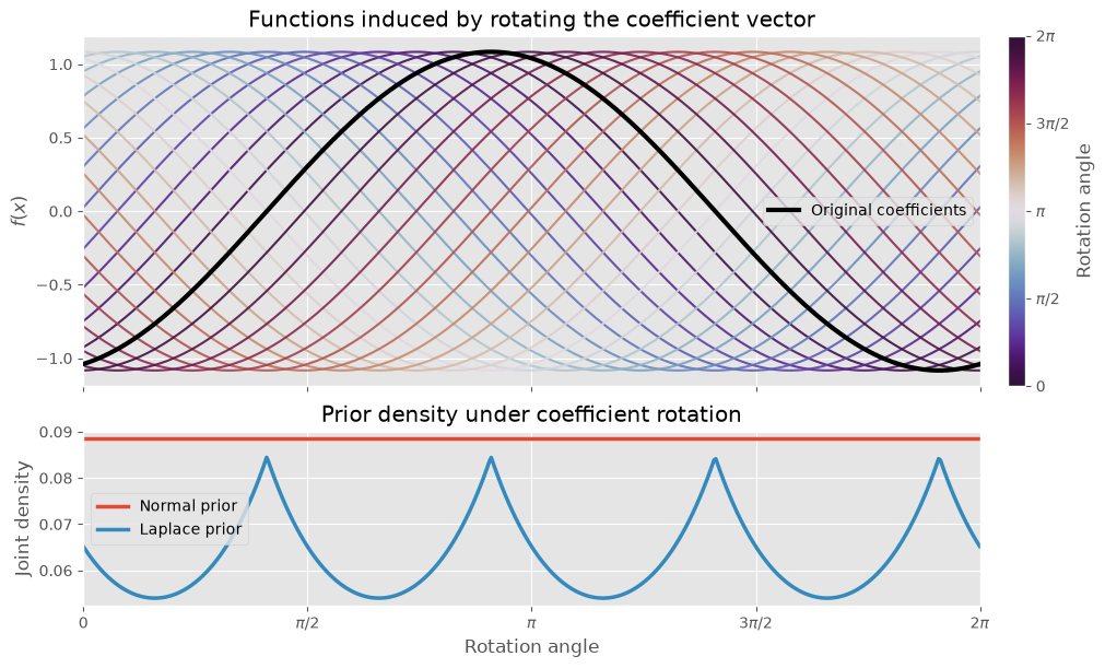
In our use case, this means that the prior for each \((a_n, b_n)\) pair should be two independent centered Gaussians with shared scale \(\sigma_n\). Specifically, setting the prior family Laplacian will encode a strong preference for certain phase shifts as seen in the figure below.

# Domain
x = np.linspace(0, 2 * np.pi, 1000)[:, None]

# Basis functions
feats = np.hstack([np.sin(x), np.cos(x)])

# Random coefficients
rng = np.random.default_rng(42)
coeffs = rng.normal(size=2)

# Angles used for displaying functions
plot_angles = np.linspace(0, 2 * np.pi, 24, endpoint=False)

# Angles used for computing the density curves
density_angles = np.linspace(0, 2 * np.pi, 500)

fig, axes = plt.subplots(
    2,
    1,
    figsize=(10, 6),
    constrained_layout=True,
    gridspec_kw={"height_ratios": [2, 1]},
)

# --------------------------------------------------------------------
# Top plot: functions
# --------------------------------------------------------------------

cmap = plt.get_cmap("twilight_shifted")
norm = mpl.colors.Normalize(vmin=0, vmax=2 * np.pi)

for angle in plot_angles:
    R = np.array([
        [np.cos(angle), -np.sin(angle)],
        [np.sin(angle),  np.cos(angle)],
    ])

    rotated_coeffs = R @ coeffs

    axes[0].plot(
        x,
        feats @ rotated_coeffs,
        color=cmap(norm(angle)),
        lw=1.5,
        alpha=0.9,
    )

# Original function
axes[0].plot(
    x,
    feats @ coeffs,
    color="black",
    lw=3,
    label="Original coefficients",
    zorder=10,
)

axes[0].set_title("Functions induced by rotating the coefficient vector")
axes[0].set_ylabel(r"$f(x)$")
axes[0].set_xlim(0, 2 * np.pi)
axes[0].set_xticks([0, np.pi / 2, np.pi, 3 * np.pi / 2, 2 * np.pi])
axes[0].set_xticklabels([])
axes[0].legend()

# Colorbar
sm = mpl.cm.ScalarMappable(norm=norm, cmap=cmap)
sm.set_array([])

cbar = fig.colorbar(
    sm,
    ax=axes[0],
    pad=0.02,
    fraction=0.05,
)

cbar.set_label("Rotation angle")
cbar.set_ticks([0, np.pi / 2, np.pi, 3 * np.pi / 2, 2 * np.pi])
cbar.set_ticklabels(
    [r"$0$", r"$\pi/2$", r"$\pi$", r"$3\pi/2$", r"$2\pi$"]
)

# --------------------------------------------------------------------
# Bottom plot: prior densities
# --------------------------------------------------------------------

normal_density = np.empty_like(density_angles)
laplace_density = np.empty_like(density_angles)

for i, angle in enumerate(density_angles):
    R = np.array([
        [np.cos(angle), -np.sin(angle)],
        [np.sin(angle),  np.cos(angle)],
    ])

    rotated_coeffs = R @ coeffs

    normal_density[i] = np.prod(stats.norm.pdf(rotated_coeffs))
    laplace_density[i] = np.prod(stats.laplace.pdf(rotated_coeffs))

axes[1].plot(
    density_angles,
    normal_density,
    color="C0",
    lw=2.5,
    label="Normal prior",
)

axes[1].plot(
    density_angles,
    laplace_density,
    color="C1",
    lw=2.5,
    label="Laplace prior",
)

axes[1].set_title("Prior density under coefficient rotation")
axes[1].set_xlabel("Rotation angle")
axes[1].set_ylabel("Joint density")

axes[1].set_xlim(0, 2 * np.pi)
axes[1].set_xticks([0, np.pi / 2, np.pi, 3 * np.pi / 2, 2 * np.pi])
axes[1].set_xticklabels(
    [r"$0$", r"$\pi/2$", r"$\pi$", r"$3\pi/2$", r"$2\pi$"]
)

axes[1].legend()

plt.show()

How to regularize

Just \(L_2\) regularize!

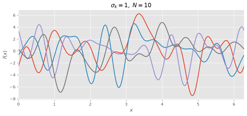
Although we have ruled out entire families of prior distributions, we still have so many different ones we could choose from. Because of the orthogonality relations described in Section 2, we have \[\lVert s_{\mathbf{a}, \mathbf{b}} \rVert_2^2 = \langle s_{\mathbf{a}, \mathbf{b}}, s_{\mathbf{a}, \mathbf{b}} \rangle = \frac{a_0^2}{2} + \sum_{n=1}^N \left(a_n^2 + b_n^2\right),\] meaning that if we set \(\sigma_1 = \sigma_2 = \dots = \sigma_N\), then we are essentially setting a prior on the \(2\)-norm of \(s\). This is pretty cool, but if you have ever tried doing this, you know that it results in very “wobbly” functions.

def fourier_basis(x, N):
    """Returns basis matrix with columns:
    sin(x), cos(x), sin(2x), cos(2x), ...
    """
    k = np.arange(1, N + 1)

    return np.column_stack([
        f
        for pair in zip(np.sin(np.outer(x, k)).T,
                        np.cos(np.outer(x, k)).T)
        for f in pair
    ])


def sample_coefficients(sigmas, n_samples, rng):
    """Sample coefficient vectors.

    sigmas : shape (2N,)
    """
    return rng.normal(scale=sigmas, size=(n_samples, len(sigmas)))


def plot_random_functions(
    basis,
    coeffs,
    x,
    ax=None,
    title=None,
):
    if ax is None:
        _, ax = plt.subplots()

    ys = coeffs @ basis.T

    ax.plot(x, ys.T, lw=2)

    ax.set_xlim(0, 2 * np.pi)
    ax.set_xlabel(r"$x$")
    ax.set_ylabel(r"$f(x)$")

    if title is not None:
        ax.set_title(title)

    return ax


# ------------------------------------------------------------

N = 10
n_samples = 4

rng = np.random.default_rng(42)

x = np.linspace(0, 2 * np.pi, 1000)

basis = fourier_basis(x, N)

# Equal variance
sigmas = np.ones(2 * N)

coeffs = sample_coefficients(sigmas, n_samples, rng)

plot_random_functions(
    basis,
    coeffs,
    x,
    title=rf"$\sigma_k=1,\; N={N}$",
)

plt.show()

A better way to do it

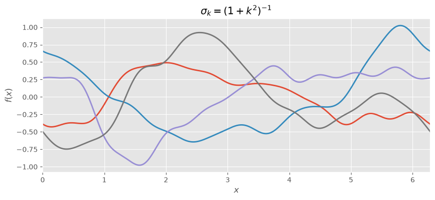
Luckily, we can do better, but we should use a different norm. Specifically, it makes intuitive sense that “penalizing wobbliness” should be related to penalizing the squared norm of the second derivative, \[\lVert s'' \rVert_2^2 = \sum_{n=1}^N n^4 \left(a_n^2 + b_n^2\right),\] instead. Note that this on its own is only a seminorm (it is blind to the constant term), so we add the \(2\)-norm back and arrive at a very special Sobolev space, \(H^2(\mathbb{T})\). Its squared norm is equivalent to \(\lVert s \rVert_2^2 + \lVert s'' \rVert_2^2\) and can be written as \[\frac{a_0^2}{2} + \sum_{n=1}^N \left(1 + n^2\right)^2 \left(a_n^2 + b_n^2\right).\]

To translate this into a prior, we will set \(\sigma_n = \frac{\sigma}{1 + n^2}\).

k = np.repeat(np.arange(1, N + 1), 2)

# H^s prior
sigmas = (1.0 + k**2) ** -1

coeffs = sample_coefficients(sigmas, n_samples, rng)

plot_random_functions(
    basis,
    coeffs,
    x,
    title=rf"$\sigma_k=(1+k^2)^{{-1}}$",
)

The “wobbliness” visibly reduced a lot and now we only really have one knob left to turn: \(\sigma\), so I consider this to be a win!

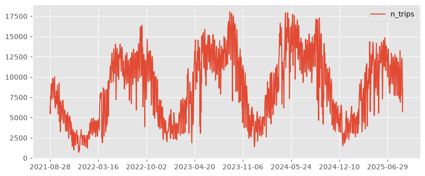
df = pd.read_csv("bubi_trips.csv", index_col=0)
df = df.iloc[100:]
df.plot()

def model(t, N=20, y=None, sobolev_prior=True):

    basis = jnp.asarray(fourier_basis(t, N))

    k = np.repeat(np.arange(1, N + 1), 2)

    A = numpyro.sample("A", dist.HalfNormal(2.0))

    if sobolev_prior:
        sigmas = A / (1 + k**2)
    else:
        sigmas = A * jnp.ones(2 * N)

    with numpyro.plate("coef", 2 * N):
        coeffs_raw = numpyro.sample(
            "coeffs_raw",
            dist.Normal(0, 1),
        )

    coeffs = numpyro.deterministic("coeffs", coeffs_raw * sigmas)

    intercept = numpyro.sample(
        "intercept",
        dist.Normal(0, 1),
    )

    slope = numpyro.sample(
        "slope",
        dist.Normal(0, 0.1),
    )

    sigma = numpyro.sample(
        "sigma",
        dist.HalfNormal(1.0),
    )

    mu = intercept + slope * (t - t.mean()) + basis @ coeffs

    numpyro.deterministic("mu", mu)

    with numpyro.plate("data", len(t)):
        numpyro.sample(
            "obs",
            dist.Normal(mu, sigma),
            obs=y,
        )

rng_key = random.key(0)
rng_key, rng_key_ = random.split(rng_key)

t = jnp.asarray((pd.to_datetime(df.index) - pd.to_datetime("2020-01-01 00:00:00")).days)
t = t / 365.25 * 2 * jnp.pi  # Convert to radians
kernel = NUTS(model)
num_samples = 2000
mcmc = MCMC(kernel, num_chains=4, num_warmup=1000, num_samples=num_samples)
y_raw = jnp.asarray(df["n_trips"].to_numpy())
y_mean, y_std = jnp.mean(y_raw), jnp.std(y_raw)
y = (y_raw - y_mean) / y_std
mcmc.run(rng_key_, t=t, y=y)

/var/folders/bp/5gg9xvvn7wj44z21_k005q3c0000gn/T/ipykernel_26733/2821868808.py:55: UserWarning: There are not enough devices to run parallel chains: expected 4 but got 1. Chains will be drawn sequentially. If you are running MCMC in CPU, consider using `numpyro.set_host_device_count(4)` at the beginning of your program. You can double-check how many devices are available in your system using `jax.local_device_count()`.
  mcmc = MCMC(kernel, num_chains=4, num_warmup=1000, num_samples=num_samples)
sample: 100%|██████████| 3000/3000 [00:04<00:00, 718.12it/s, 63 steps of size 6.96e-02. acc. prob=0.91] 
sample: 100%|██████████| 3000/3000 [00:03<00:00, 811.89it/s, 63 steps of size 6.50e-02. acc. prob=0.94] 
sample: 100%|██████████| 3000/3000 [00:10<00:00, 292.76it/s, 63 steps of size 5.55e-02. acc. prob=0.95]
sample: 100%|██████████| 3000/3000 [00:03<00:00, 763.00it/s, 63 steps of size 6.26e-02. acc. prob=0.94] 

idata = mcmc.get_samples()

Comparison with a plain Normal prior

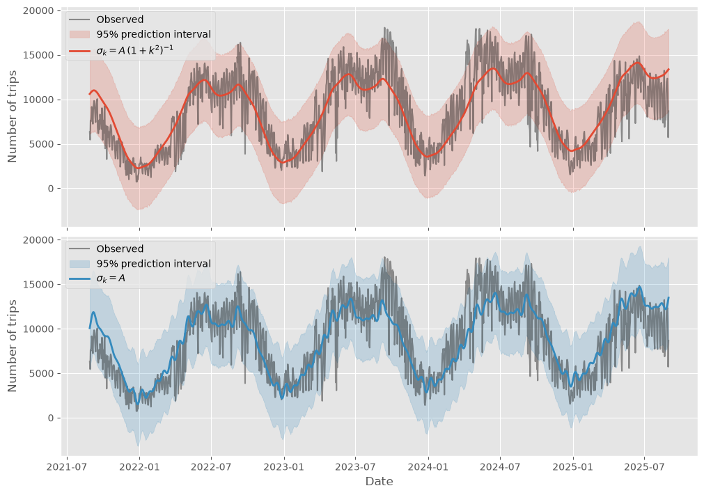
To see what the \((1 + k^2)^{-1}\) scaling actually buys us, let’s fit the exact same model with a plain Normal prior, that is, with \(\sigma_1 = \dots = \sigma_N = A\). This is the equal-variance prior from before, which only constrains the \(2\)-norm of the seasonal component.

mcmc_flat = MCMC(NUTS(model), num_chains=4, num_warmup=1000, num_samples=num_samples)

rng_key, rng_key_ = random.split(rng_key)
mcmc_flat.run(rng_key_, t=t, y=y, sobolev_prior=False)

idata_flat = mcmc_flat.get_samples()

/var/folders/bp/5gg9xvvn7wj44z21_k005q3c0000gn/T/ipykernel_26733/3212244970.py:1: UserWarning: There are not enough devices to run parallel chains: expected 4 but got 1. Chains will be drawn sequentially. If you are running MCMC in CPU, consider using `numpyro.set_host_device_count(4)` at the beginning of your program. You can double-check how many devices are available in your system using `jax.local_device_count()`.
  mcmc_flat = MCMC(NUTS(model), num_chains=4, num_warmup=1000, num_samples=num_samples)
sample: 100%|██████████| 3000/3000 [00:02<00:00, 1210.57it/s, 31 steps of size 1.22e-01. acc. prob=0.94]
sample: 100%|██████████| 3000/3000 [00:03<00:00, 912.64it/s, 31 steps of size 1.06e-01. acc. prob=0.95] 
sample: 100%|██████████| 3000/3000 [00:02<00:00, 1025.87it/s, 31 steps of size 1.37e-01. acc. prob=0.93]
sample: 100%|██████████| 3000/3000 [00:01<00:00, 1591.88it/s, 31 steps of size 1.26e-01. acc. prob=0.93]

rng = np.random.default_rng(0)

dates = pd.to_datetime(df.index)

fig, axes = plt.subplots(
    2,
    1,
    figsize=(10, 7),
    sharex=True,
    sharey=True,
    constrained_layout=True,
)

for ax, samples, color, label in [
    (axes[0], idata, "C0", r"$\sigma_k = A \, (1 + k^2)^{-1}$"),
    (axes[1], idata_flat, "C1", r"$\sigma_k = A$"),
]:
    # Back to the original scale (number of trips)
    mu = np.asarray(samples["mu"]) * float(y_std) + float(y_mean)
    sigma = np.asarray(samples["sigma"])[:, None] * float(y_std)

    # Posterior predictive draws: add observation noise to each mu sample
    y_rep = mu + sigma * rng.normal(size=mu.shape)
    lower, upper = np.percentile(y_rep, [2.5, 97.5], axis=0)

    ax.plot(dates, np.asarray(y_raw), alpha=0.4, color="black", label="Observed")
    ax.fill_between(
        dates,
        lower,
        upper,
        color=color,
        alpha=0.2,
        label="95% prediction interval",
    )
    ax.plot(dates, mu.mean(axis=0), lw=2, color=color, label=label)

    ax.set_ylabel("Number of trips")
    ax.legend(loc="upper left")

axes[1].set_xlabel("Date")

plt.show()